November 20, 2019
Micropolitics of a Recommender System – Source Code
Introduction
This text aims to explain some of the source code of the open source recommender system LightFM. This piece of software was originally developed by Maciej Kula while working as a data scientist for the online fashion store Lyst, who aggregates millions of products from across the web. It was written with the aim of recommending fashion products from this vast catalogue based to users with few or no prior interactions with Lyst.1Cp. Maciej Kula, “Metadata Embeddings for User and Item Cold-start Recommendations”, paper presented in the 2nd Workshop on New Trends on Content-Based Recommender Systems co-located with 9th ACM Conference on Recommender Systems, 2015. Available at: http://ceur-ws.org/Vol-1448/paper4.pdf [accessed July 27, 2018]. At the time of writing, LightFM is still under active development by Kula with minor contributions from 17 other developers over the past three years. The repository is moderately popular, having been starred by 2,032 GitHub users; 352 users have forked the repository, creating their own version of it that they can modify.2Cp. Maciej Kula, “GitHub – lyst/lightfm: A Python implementation of LightFM, a hybrid recommendation algorithm”, posted to Github. Available at: https://github.com/lyst/lightfm [accessed November 4, 2018]. Users have submitted 233 issues, such as error reports and feature requests to LightFM over the course of its existence, which suggests a modest but active community of users.3Cp. Maciej Kula, “Issues – lyst/lightfm – GitHub”, posted to Github. Available at: https://github.com/lyst/lightfm/issues [accessed November 4, 2018]. To put these numbers in perspective, the most popular machine learning framework on Github, Tensorflow, has been starred 113,569 times and forked 69,233 times with 14,306 issues submitted.4Cp. TensorFlow, “GitHub – tensorflow/tensorflow: An Open Source Machine Learning Framework for Everyone”, posted to Github. Available at: https://github.com/tensorflow/tensorflow [accessed November 4, 2018].
While the theoretical text that accompanies this one addresses aspects of machine learning in LightFM, none of the source code quoted here actually does any machine learning. Instead, the examples here are chosen to demonstrate how an already trained model is processed so as to arrive at recommendations. The machine learning aspect of LightFM can be briefly explicated using Tim Mitchell’s much-cited definition: “A computer program is said to learn from experience E with respect to some class of tasks T and performance measure P, if its performance at tasks in T, as measured by P improves with experience E.”5Tom Mitchell, Machine Learning, London, McGraw-Hill, 1997, p. 2. Task T, in this case, is recommending products to users that they are likely to buy. E is historical data on interactions between users and products as well as metadata about those users and products. P is the extent to which the model’s predictions match actual historical user-item interactions
In practice, P is represented by a number produced by a loss function (also known as cost function or objective function) that outputs higher numbers for poorly performing models whose predictions don’t match historical data. To arrive at an effective model, P needs to be minimised through some usually iterative process, which in the case of LightFM is a form of gradient descent.6Cp. Kula, “Metadata Embeddings for User and Item Cold-start Recommendations”. Gradient descent begins with a model with random, fairly arbitrary parameters and repeatedly tests the model, each time changing the parameters slightly with the aim of reducing the model loss (the number output by the loss function) and eventually reaching an optimal set of parameters.7Cp. Andrew Ng, “Lecture 2.5 — Linear Regression With One Variable | Gradient Descent — [ Andrew Ng]”, lecture posted to Youtube. Available at: https://www.youtube.com/watch?v=F6GSRDoB-Cg [accessed November 4, 2018]. The parameters of LightFM’s model are embedding vectors for each feature or category that may be applied to a user or item; these are discussed in greater detail below. Returning to Mitchel’s definition: as gradient descent only optimises the model based on the historical data available, it is clear that up to a certain point, LightFM is likely to produce more relevant recommendations (T) if it is trained using a larger and presumably more representative set of test and training data (E).
The below excerpts of source code are taken from a file in the LightFM Git repository named _lightfm_fast.pyx.template. This file defines most of the actual number-crunching carried out by the LightFM recommender and is written in Cython, a special form of Python that works like a template for generating C code. The file contains 1,386 lines of Cython and is used to generate up to 30,720 lines of C. While verbose to us, this generated C code is compiled into even more prolix machine code which computers execute much faster than Python. Both examples are function definitions; they start with the word ‘cdef’ which in this case indicates that the definition of a function that can be compiled into C is to follow. Functions take input data in the form of one or more arguments and perform some computation using these data. They either modify the data that is passed into them or output some new data derived from this input. In the case of compute_representation, the word ‘void’ precedes the function name, indicating that the function outputs or returns nothing and would be expected to do something to its input. In the second example the word ‘flt’ (an alias for ‘float’) precedes compute_prediction_from_repr, meaning that it is expected to return a floating point number. For brevity’s sake, a floating point number is basically a decimal like 1.6.
Function 1: compute_representation8Maciej Kula, “lightfm/_lightfm_fast.pyx.template”, posted to Github, line 287. Availabe at: https://github.com/lyst/lightfm/blob/e12cfc7e5fa09c1694b98acc96af3ed2754646ae/lightfm/_lightfm_fast.pyx.template#L287 [accessed July 25, 2018].
This function is responsible for taking data about users (e.g. customers) and items (e.g. clothes or films) and producing latent representations of them. These representations can be used by the second function ‘compute_prediction_from_repr’ to predict the level of affinity between these users and items.
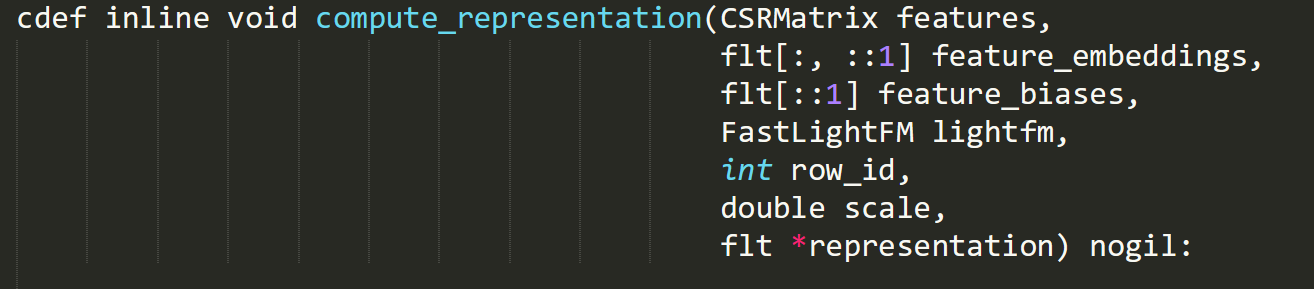
The comma-separated lines in parentheses following the name of the function above are parameter declarations; these determine what data or arguments can be passed into the function. The first part of each parameter declaration can be thought of as the type of the expected argument and the second part is the name used to reference it in the body of the function. Here is an explanation of each of the parameters:
- features: an object belonging to the class ‘CSRMatrix’. Matrices are like tables, or row-column addressable grids, whose cells contain numbers. CSR matrices offer a way of storing matrices in which most of the numbers are zero; in other words: when the matrices are sparse. In this case – sticking with the table analogy – the rows correspond to users or items and the columns correspond to features of these users or items. If the items are films, each feature could be a genre. Cells in the table might contain 1 if the film (row) belonged to genre (column) and 0 if it didn’t. Each row in the matrix can be taken as a vector representing the corresponding film.
- feature_embeddings: a two-dimensional array, which is also like a table with rows and columns. This array contains the embeddings for features that have been learned from training data using gradient descent, as discussed above. This array has a row for each feature and a column for each dimension of the features’ embeddings. These feature embedding rows can be thought of as vectors that contain information about how similar each feature is to others based on shared positive user interactions such as favourites and purchases. Vectors are like arrows with a direction and a magnitude or length. The row vectors of the ‘feature_embeddings’ array are represented by their Cartesian coordinates, such that if each row contained two numbers, the vectors would be two-dimensional and the first number might specify the horizontal position of the end of the vector (the tip of the arrow) and the second number the vertical position. If two features (e.g. ‘action’ and ‘adventure’ or ‘black’ and ‘dress’) are shared by items bought by the same 1,000 users, their embeddings will be similar; they will point in a similar direction. To illustrate: the similarity of two two-dimensional feature embeddings could be worked out by plotting them both on a sheet of paper as arrows originating from the same point and measuring the shortest angle between them using a protractor; the smaller this angle, the greater the affinity between the features.
- feature_biases: a one-dimensional array of floating point numbers. This is like a list of decimal numbers.
- lightfm: an object of the class FastLightFM. This object holds information about the state of the recommender model.
- row_id: an integer, or whole number, identifying the row in the features matrix that the function should compute a representation for.
- Scale: a double-precision floating point number. It is called double-precision because it takes up 64 bits, or binary digits, of memory rather than the standard 32.
- representation: reference to a one-dimensional array of floating-point numbers. When executed, the ‘compute_representation’ function modifies the contents of the referenced ‘representation’ array.
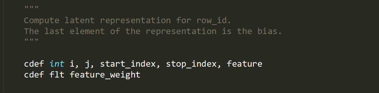
The two lines above are declaring variables, which allow a value of a particular type to be referenced by a name such as ‘start_index’. All of these variables are numbers that are used later in the function.

Two of the variables declared above are being assigned values that are returned by the ‘get_row_start’ and ‘get_row_end’ functions. These functions are part of the ‘features’ CSRMatrix object and are called methods.

The above two lines comprise a simple Python for-loop. The loop counts up from zero to the value of ‘lightfm.no_components + 1’ in increments of one, each time setting the value of variable ‘i’ to the current count. For each increment it executes the indented code ‘representation[i] = 0.0’, which sets the ith element of the ‘representation’ array to zero. In effect, it sets every number in ‘representation’ to zero.
Note: ‘lightfm.no_components’ is an integer that determines the dimensionality of the features’ latent embeddings. If ‘no_components’ is ‘10’, each feature is represented by a ten-dimensional vector.

This for-loop is slightly different, it counts up from ‘start_index’ to ‘stop_index’, setting ‘i’ to the current count each time. It also executes five lines of indented code upon each iteration, including another nested for-loop. The following two lines set the ‘feature’ and ‘feature_weight’ variables to the appropriate values from the CSR matrix object. ‘feature’ is set to the index of the feature ‘i’, as stored in the ‘feature_embeddings’ array. ‘feature_weight’ is set to a value that indicates whether this particular feature belongs to the user or item the ‘compute_repr’ function computing is a representation for; this is probably ‘1’ if the feature belongs and ‘0’ if it doesn’t.
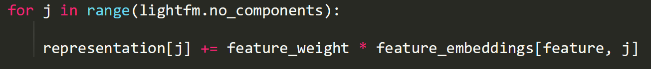
This nested for-loop counts from zero to the number of components (the dimensionality of the feature embedding) in increments of one and sets j to the current count. ‘feature_weight’ will maintain the same value for the duration of the loop: either ‘1’ or ‘0’. This means that either the entire feature embedding will be added to the ‘representation’ array or none of it.
All this loop is doing is adding together the latent representations of the features of a given item or user. As Maciej Kula puts it: “The representation for denim jacket is simply a sum of the representation of denim and the representation of jacket; the representation for a female user from the US is a sum of the representations of US and female users.”9Cp. Kula, “Metadata Embeddings for User and Item Cold-start Recommendations”.

If the user or item has the feature ‘features.data[i]’, that feature’s bias is added to the final bias element of the ‘representation’ array.
Function 2: compute_prediction_from_repr10Maciej Kula, “lightfm/_lightfm_fast.pyx.template”, posted to Github, line 320. Available at: https://github.com/lyst/lightfm/blob/e12cfc7e5fa09c1694b98acc96af3ed2754646ae/lightfm/_lightfm_fast.pyx.template#L320 [accessed July 25, 2018].
This function is responsible for predicting how likely a user is to be interested in an item.
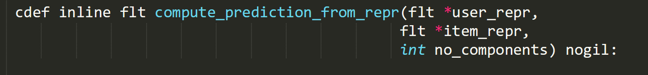
There are only three parameters this time:
- user_repr: a reference to a one-dimensional array of floating point numbers. Its contents will have been produced by the ‘compute_representation’ function above based on the features and other data for a user.
- item_repr: a reference to a representation of the features of a given item, also produced by the ‘compute_representation’ function.
- no_components: the number of dimensions of the representation vectors.

The variable ‘result’ is set to the sum of the bias component of the latent representations for both the user and item.
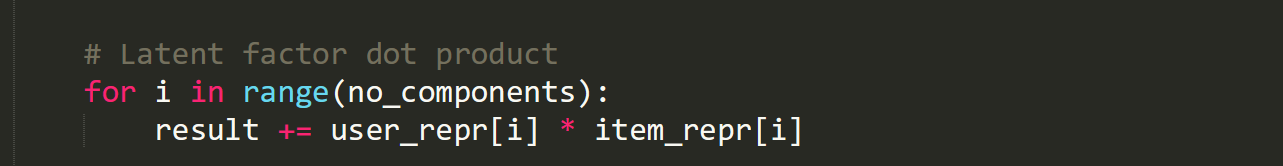
This loop adds the dot product or inner product of the user’s and item’s representation vectors to the ‘result’ vector. The dot product of two vectors is the sum of the results of multiplying each part of the first vector by the corresponding part of the second vector, as can be seen in the loop: ‘user_repr[i] * item_repr[i]’.
The dot product is a single number that varies with the difference in direction between the embedding vectors ‘user_repr’ and ‘item_repr’ and is greater if they are facing the same way. As these embeddings have been calculated based on known interactions between users and items, the dot product gives an indication of how likely any user is to interact positively with any item.

The function returns the dot product added to the sum of the item and user’s biases. These biases are calculated in the ‘compute_representation’ function and are the sums of the biases of the item and user’s active feature. This effectively gives LightFM the ability to treat some features as more important than others.
| ↑1 | Cp. Maciej Kula, “Metadata Embeddings for User and Item Cold-start Recommendations”, paper presented in the 2nd Workshop on New Trends on Content-Based Recommender Systems co-located with 9th ACM Conference on Recommender Systems, 2015. Available at: http://ceur-ws.org/Vol-1448/paper4.pdf [accessed July 27, 2018]. |
|---|---|
| ↑2 | Cp. Maciej Kula, “GitHub – lyst/lightfm: A Python implementation of LightFM, a hybrid recommendation algorithm”, posted to Github. Available at: https://github.com/lyst/lightfm [accessed November 4, 2018]. |
| ↑3 | Cp. Maciej Kula, “Issues – lyst/lightfm – GitHub”, posted to Github. Available at: https://github.com/lyst/lightfm/issues [accessed November 4, 2018]. |
| ↑4 | Cp. TensorFlow, “GitHub – tensorflow/tensorflow: An Open Source Machine Learning Framework for Everyone”, posted to Github. Available at: https://github.com/tensorflow/tensorflow [accessed November 4, 2018]. |
| ↑5 | Tom Mitchell, Machine Learning, London, McGraw-Hill, 1997, p. 2. |
| ↑6 | Cp. Kula, “Metadata Embeddings for User and Item Cold-start Recommendations”. |
| ↑7 | Cp. Andrew Ng, “Lecture 2.5 — Linear Regression With One Variable | Gradient Descent — [ Andrew Ng]”, lecture posted to Youtube. Available at: https://www.youtube.com/watch?v=F6GSRDoB-Cg [accessed November 4, 2018]. |
| ↑8 | Maciej Kula, “lightfm/_lightfm_fast.pyx.template”, posted to Github, line 287. Availabe at: https://github.com/lyst/lightfm/blob/e12cfc7e5fa09c1694b98acc96af3ed2754646ae/lightfm/_lightfm_fast.pyx.template#L287 [accessed July 25, 2018]. |
| ↑9 | Cp. Kula, “Metadata Embeddings for User and Item Cold-start Recommendations”. |
| ↑10 | Maciej Kula, “lightfm/_lightfm_fast.pyx.template”, posted to Github, line 320. Available at: https://github.com/lyst/lightfm/blob/e12cfc7e5fa09c1694b98acc96af3ed2754646ae/lightfm/_lightfm_fast.pyx.template#L320 [accessed July 25, 2018]. |

Simon Crowe is a programmer, researcher and artist. He was awarded a master’s degree in Digital Culture by Goldsmiths University of London in 2017, after which he stayed on at Goldsmiths for a year as a Visiting Researcher. His research deals with the relationship between data-driven predictive models and questions of power, control and agency in digital cultures.